Asymptotic Notations
- Asymptotic notation is useful describe the running time of the algorithm.
- Asymptotic notations give time complexity as “fastest possible”, “slowest possible” or “average time”.
- Asymptotic notation is useful because it allows us to concentrate on the main factor determining a functions growth.
Following are commonly used asymptotic notations used in calculating running time complexity of an algorithm.
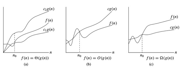
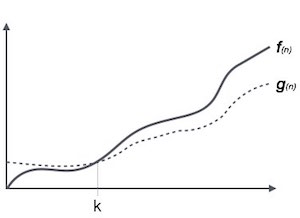
1.Big O notation (upper bound –worst Case)
- The Ο(n) is the formal way to express the upper bound of an algorithm’s running time.
- It always indicates the maximum time required by an algorithm for all input values.
- That means Big – Oh notation describes the worst case of an algorithm time complexity.
Definition: O(g(n)) = {f(n) : there exists positive constants c and n0 such that 0 ≤ f(n) ≤ c g(n) for all n ≥ n0.

2. Omega notation (lower bound- best case )
- omega notation provides an asymptotic lower bound on a function.
- It measures the best case time complexity or best amount of time an algorithm can possibly take to complete.
-
1Ω(<i>f</i>(n)) ≥ { <i>g</i>(n) : there exists c > 0 and n<sub>0</sub> such that <i>g</i>(n) ≤ c.<i>f</i>(n) for all n > n<sub>0</sub>. }
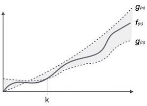
3. Theta (θ)notation (upper bound as well as lower bound – Average case )
- The θ(n) is the formal way to express both the lower bound and upper bound of an algorithm’s running time.
- It measures the Average case Complexity.
|
1 |
θ(<i>f</i>(n)) = { <i>g</i>(n) if and only if <i>g</i>(n) = Ο(<i>f</i>(n)) and <i>g</i>(n) = Ω(<i>f</i>(n)) for all n > n<sub>0</sub>. } |
Common Asymptotic Notations
Following is a list of some common asymptotic notations −
| constant | − | Ο(1) |
| logarithmic | − | Ο(log n) |
| linear | − | Ο(n) |
| n log n | − | Ο(n log n) |
| quadratic | − | Ο(n2) |
| cubic | − | Ο(n3) |
| polynomial | − | nΟ(1) |
| exponential | − | 2Ο(n) |
P,NP & NP completeness
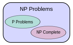
- Class P
P is a complexity class that represents the set of all decision problems that can be solved in polynomial time. That is, given an instance of the problem, the answer yes or no can be decided in polynomial time. “P” stands for “polynomial time.”
- Class NP
The term “NP” stands for “nondeterministic polynomial” .NP is a complexity class that represents the set of all decision problems for which the instances where the answer is “yes” have proofs that can be verified in polynomial time .Eg. Sudoku, chess game
-
- Class NP-Complete
NP-Complete is a complexity class which represents the set of all problems X in NP for which it is possible to reduce any other NP problem Y to X in polynomial time.
- Class NP-hard
The term NP-hard refers to any problem that is at least as hard as any problem in NP. Thus, the NP-complete problems are precisely the intersection of the class of NP-hard problems with the class NP
Amortized Complexity
An amortized analysis is any strategy for analyzing a sequence of operations to show that the average cost per operation is small, even though a single operation within the sequence might be expensive.Even though we’re taking averages, however, probability is not involved.In an amortized analysis, the time required to perform a sequence of data structure operations is averaged over all the operations performed.
Amortized analysis differs from average-case analysis in that probability is not involved; an amortized analysis guarantees the average performance of each operation in the worst case.
- A. Aggregate method
- B. The accounting method
- C. The potential method
- D. Dynamic tables
A) Aggregate Method
The aggregate method is used to find the total cost. If we want to add a bunch of data, then we need to find the amortized cost by this formula.
For a sequence of n operations, the cost is −

Aggregate Method Characteristics
- It computes the worst case time T(n) for a sequence of n operations.
- The amortized cost is T(n)/n per operation.
- It gives the average performance of each operation in the worst case.
- This method is less precise than other methods, as all operations are assigned the same cost.
B) Accounting Method
- In the accounting method of amortized analysis, we assign differing charges to different operations, with some operations charged more or less than they actually cost.
- The amount we charge an operation is called its amortized cost.
- When an operation’s amortized cost exceeds its actual cost, the difference is assigned to specific objects in the data structure as credit.
- Credit can be used later on to help pay for operations whose amortized cost is less than their actual cost. Thus, one can view the amortized cost of an operation as being split between its actual cost and credit that is either deposited or used up.
- This method is very different from aggregate analysis, in which all operations have the same amortized cost.
- we overcharge some operations early and use them to as prepaid charge later.
- One must choose the amortized costs of operations carefully. If we want analysis with amortized costs to show that in the worst case the average cost per operation is small, the total amortized cost of a sequence of operations must be an upper bound on the total actual cost of the sequence. Moreover, as in aggregate analysis, this relationship must hold for all sequences of operations. If we denote the actual cost of the ith operation by ci and the amortized cost of the ith operation by , we require
c) Potential Method
- According to computational complexity theory, the potential method is defined as a method implemented to analyze the amortized time and space complexity of a data structure, a measure of its performance over sequences of operations that eliminates the cost of infrequent but expensive operations.In the potential method, a function Φ is selected that converts states of the data structure to non-negative numbers. If S is treated as state of the data structure, Φ(S) denotes work that has been accounted in the amortized analysis but not yet performed. Thus, Φ(S) may be imagined as calculating the amount of potential energy stored in that state. Before initializing a data structure, the potential value is defined to be zero. Alternatively, Φ(S) may be imagined as representing the amount of disorder in state S or its distance from an ideal state.
Applications of amortized analysis
- Vectors/ tables
- Disjoint sets
- Priority queues
- Heaps, Binomial heaps, Fibonacci heaps
- Hashing