Sorting refers to the operation or technique of arranging and rearranging sets of data in some specific order. A collection of records called a list where every record has one or more fields. The fields which contain a unique value for each record is termed as the key field. For example, a phone number directory can be thought of as a list where each record has three fields – ‘name’ of the person, ‘address’ of that person, and their ‘phone numbers’. Being unique phone number can work as a key to locate any record in the list.
Sorting is the operation performed to arrange the records of a table or list in some order according to some specific ordering criterion. Sorting is performed according to some key value of each record.

Categories of Sorting

The techniques of sorting can be divided into two categories. These are:

Internal Sorting
External Sorting

Internal Sorting: If all the data that is to be sorted can be adjusted at a time in the main memory, the internal sorting method is being performed.
External Sorting: When the data that is to be sorted cannot be accommodated in the memory at the same time and some has to be kept in auxiliary memory such as hard disk, floppy disk, magnetic tapes etc, then external sorting methods are performed.

Types of Sorting

Elementary Sorting Algorithms

Bubble sort
Selection sort
Insertion Sort

Efficient Sorting Algorithm

Quick sort
Merge Sort
Heap sort
Radix sort

1. Bubble Sort

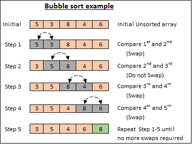
In bubble sort we compare 2 items at a time, and we either swap them or move on to compare the next pair. It is infamously slow, but it’s conceptually the simplest of the sorting algorithm.

2nd example
../_images/bubblepass.png
3rd example
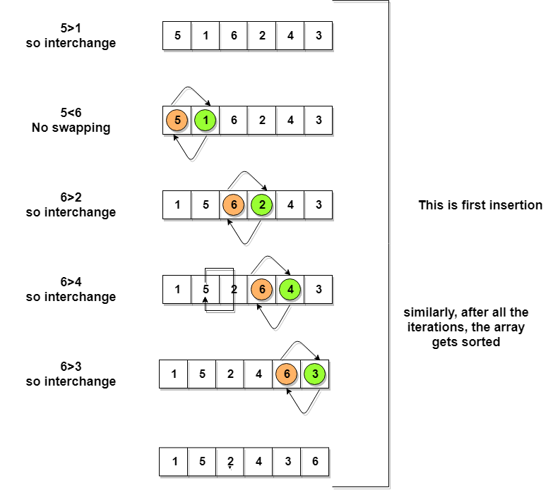
Let’s consider an array with values {5, 1, 6, 2, 4, 3}
Below, we have a pictorial representation of how bubble sort will sort the given array.
Bubble sort algorithm

public void bubbleSort() {
int out, in, temp;
int[] a = new int[nElems]; // nElems is the number of elements we'll input later ^^||
for(out=nElems-1; out>1; out--) {
for(in=0; in<out; in++) {
if( a[in] > a[in+1] ) { // out of order?
temp = a[in]; // swap them
a[in] = a[in+1];
a[in+1] = temp;
}
}
}
}

public void bubbleSort() {

int out, in, temp;

int[] a = new int[nElems]; // nElems is the number of elements we'll input later ^^||

for(out=nElems-1; out>1; out--) {

for(in=0; in<out; in++) {

if( a[in] > a[in+1] ) { // out of order?

temp = a[in]; // swap them

a[in] = a[in+1];

a[in+1] = temp;

}

Following are the Time and Space complexity for the Bubble Sort algorithm.

Worst Case Time Complexity [ Big-O ]: O(n²)
Best Case Time Complexity [Big-omega]: O(n)
Average Time Complexity [Big-theta]: O(n²)
Space Complexity: O(1)

2. Selection Sort

In selection sort, we move along the data and select the smallest item, swap the selected item to the position 0, and so on.

public void bubbleSort() {
int out, in, temp;
int[] a = new int[nElems]; // nElems is the number of elements we'll input later ^^||
for(out=nElems-1; out>1; out--) public void selectionSort() {
int out, in, min, temp;
int[] a = new int[nElems]; // nElems is the number of elements we'll input later ^^||
for(out=0; out<nElems-1; out++) {
min = out;
for(in = out+1; in<nElems; in++) {
if(a[in] < a[min]) { // if min is greater,
min = in; // we have a new min
temp = a[out]; // swap 'em
a[out] = a[min];
a[min] = temp;
}
}
}
}
}

public void bubbleSort() {

int out, in, temp;

int[] a = new int[nElems]; // nElems is the number of elements we'll input later ^^||

for(out=nElems-1; out>1; out--) public void selectionSort() {

int out, in, min, temp;

int[] a = new int[nElems]; // nElems is the number of elements we'll input later ^^||

for(out=0; out<nElems-1; out++) {

min = out;

for(in = out+1; in<nElems; in++) {

if(a[in] < a[min]) { // if min is greater,

min = in; // we have a new min

temp = a[out]; // swap 'em

a[out] = a[min];

a[min] = temp;

}

Complexity Analysis of Selection Sort

Selection Sort requires two nested for loops to complete itself, one for loop is in the function selectionSort, and inside the first loop we are making a call to another function indexOfMinimum, which has the second(inner) for loop.
Hence for a given input size of n, following will be the time and space complexity for selection sort algorithm:

Worst Case Time Complexity [ Big-O ]: O(n²)
Best Case Time Complexity [Big-omega]: O(n²)
Average Time Complexity [Big-theta]: O(n²)
Space Complexity: O(1)

3. Insertion Sort

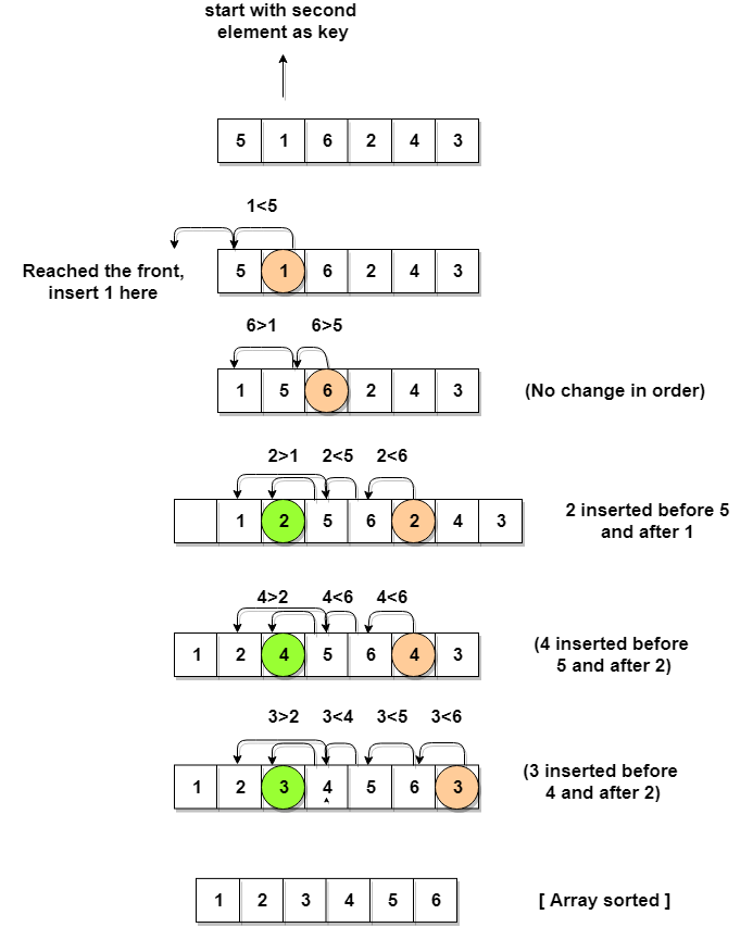
We divide the data into 2 lists (sorted and unsorted). In each iteration, the first element of the unsorted list is inserted at appropriate position into the sorted list.

2nd example :-
Insertion Sort algorithm pictorial representation

Complexity Analysis of Insertion Sort

Worst Case Time Complexity [ Big-O ]: O(n²)
Best Case Time Complexity [Big-omega]: O(n)
Average Time Complexity [Big-theta]: O(n²)
Space Complexity: O(1)

public void insertionSort() {
int in, out;
int[] a = new int[nElems]; // nElems is the number of elements we'll input later ^^||
for(out=1; out<nElems; out++) { // out is dividing line
long temp = a[out]; // remove marked item
in = out; // start shifts at out
while(in>0 && a[in-1]>=temp) { // until one is smaller,
a[in] = a[in-1]; // shift item to right
--in; // go left one position
}
a[in] = temp; // insert marked item
}
}

public void insertionSort() {

int in, out;

int[] a = new int[nElems]; // nElems is the number of elements we'll input later ^^||

for(out=1; out<nElems; out++) { // out is dividing line

long temp = a[out]; // remove marked item

in = out; // start shifts at out

while(in>0 && a[in-1]>=temp) { // until one is smaller,

a[in] = a[in-1]; // shift item to right

--in; // go left one position

}

a[in] = temp; // insert marked item

}

Comparing the 3 simple sorts

They require only their initial data array plus a little extra memory, but all their algorithms execute in O(N²) time.

The bubble sort is simple, but the least efficient. It is practical if the amount of data is small
The selection sort minimizes the number of swaps, but the number of comparisons is still high
The insertion sort is the most versatile of the three, and is the best in most situations, assuming the amount of data is small or the data is almost sorted.

Efficient Sorting Algorithm

Merge Sort Algorithm

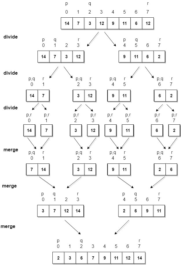
Merge Sort follows the rule of Divide and Conquer to sort a given set of numbers/elements, recursively, hence consuming less time.
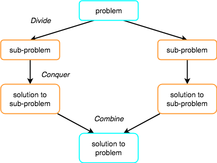
Divide and Conquer :- If we can break a single big problem into smaller sub-problems, solve the smaller sub-problems and combine their solutions to find the solution for the original big problem, it becomes easier to solve the whole problem.
The concept of Divide and Conquer involves three steps:

Divide the problem into multiple small problems.
Conquer the subproblems by solving them. The idea is to break down the problem into atomic subproblems, where they are actually solved.
Combine the solutions of the subproblems to find the solution of the actual problem

Divide and Conquer algorithm
1st example
../_images/mergesortA.png
../_images/mergesortB.png
2nd example
Let’s consider an array with values {14, 7, 3, 12, 9, 11, 6, 12}
Below, we have a pictorial representation of how merge sort will sort the given array.
Working of Merge Sort algorithm

The Quick Sort

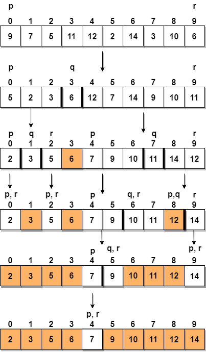
The quick sort uses divide and conquer to gain the same advantages as the merge sort, while not using additional storage. As a trade-off, however, it is possible that the list may not be divided in half. When this happens, we will see that performance is diminished.
A quick sort first selects a value, which is called the pivot value. Although there are many different ways to choose the pivot value, we will simply use the first item in the list. The role of the pivot value is to assist with splitting the list. The actual position where the pivot value belongs in the final sorted list, commonly called the split point, will be used to divide the list for subsequent calls to the quick sort.
1st example :-
../_images/partitionA.png
2nd example :-
How Quick Sort algorithm works

Heap Sort Algorithm

Heap Sort is one of the best sorting methods being in-place and with no quadratic worst-case running time. Heap sort involves building a Heap data structure from the given array and then utilizing the Heap to sort the array.

What is a Heap ?

Heap is a special tree-based data structure, that satisfies the following special heap properties:

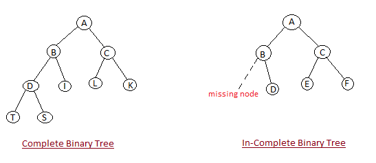
Shape Property: Heap data structure is always a Complete Binary Tree, which means all levels of the tree are fully filled.
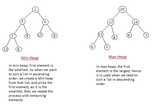
Heap Property: All nodes are either greater than or equal to or less than or equal to each of its children. If the parent nodes are greater than their child nodes, heap is called a Max-Heap, and if the parent nodes are smaller than their child nodes, heap is called Min-Heap.